Title: Design Considerations for a Ground-Based Search for Transiting Planets around L and T Dwarfs
Authors: Patrick Tamburo, Philip S. Muirhead
First Author’s Institution: Boston University Department of Astronomy, Boston, MA, USA
Status: Accepted to PASP
Over the last 20 or so years, over 3000 exoplanets have been detected, most around stars like our Sun. Recently, many exoplanet hunters have been focusing on M dwarfs, as Earth-sized planets at habitable temperatures are easier to detect. But could we go even cooler? L and T dwarfs (LTs) are a mixed bunch. While all have radii about 1 RJup and temperatures 500-2200 K, their masses vary wildly from stellar main sequence (0.08MSun) through brown dwarfs to planetary mass objects. Earth around a L0 star would produce transits blocking 1% of their host star’s light and receive the same amount of flux orbiting in just 1.65 days, making the habitable zone even more accessible. The habitable zone may actually be further out due to tidal heating, as happens to Jupiter’s moon Io.
But can these planets exist? Theory and observations suggest so. Circumstellar disks, from which planets form, have been observed around M-type brown dwarfs and 3 MJup objects have been detected around brown dwarfs at large separation by direct imaging. While slightly higher mass, TRAPPIST-1 is the prime example of an ultracool M8 dwarf with 7 Earth-sized planets. Theory suggests that brown dwarfs may be able to form planets up to 5 Earth masses, and considering planets are very common around M dwarfs, perhaps it is reasonable to expect planets around LTs.
Discovering planets around LTs would inform our general theory on satellite formation and help us understand how planet occurrence rates vary compared to higher mass stars and within the wide range of LTs. Astronomers are also interested whether planets around LTs are predominately terrestrial. So what is the best way to search for them?
(Simulated) battle of the bands
We have not observed transits for L and T dwarfs because seeing the ~1% dimming is much harder for faint objects. These very red objects are brightest in the infrared but infrared detectors are less sensitive than optical when observing through the Earth’s atmosphere. The authors measured the sky brightness of real detectors in: the red optical z’ band; J , H and K bands using near infrared detectors and repeated J and K bands using high dark current InGaAs detectors, which are cheaper.
They compared the six different bands by simulating photometry for a large sample of LTs, assuming a 2m telescope and 30 second exposures. Figure 1 shows the signal and noise levels for a lightcurve combining data, or binning, to one hour (the expected transit time of a habitable zone planet). Figure 1 shows that the H band has the lowest amount of scatter, so where the brightest part of the LTs spectrum is more than compensates for the higher sky background. Looking at the median brightness star, the smallest planet which is strongly detected (at 7.1 σ) around a typical LT is 0.60 REarth, provided that when the data is binned, the transit is fully contained within one bin. Step 1 complete: H band is best to observe LTs and is sensitive to Earth-sized planets across the range of magnitudes, although this does not account for systematic noise.
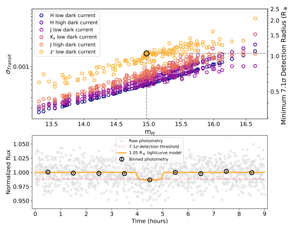
Figure 1: Top: Photometric error across LT brightness, as measured in the H band. Errors for all six detectors and the corresponding minimum detection radius for a 7.1 σ detection around a typical LT of 0.88 RJup is shown. Scatter in H band is 2.7x smaller than for z’ band. Bottom: Example of an injected transit shows the minimum detection radius in the z’ band is 1.05 REarth for the median brightness star. Figure 1 from today’s paper.
Simulating the LTs
Time to simulate some planetary systems and work out which can be retrieved! They first checked how many LTs were visible from their test location of the 1.8m Perkins telescope in Arizona, finding 998 were. They assumed 10 nights observing per month for a period of 1-5 years and scheduled targets which were visible for a large fraction of the night.
The authors assigned system properties to each of the 998 visible LTs, finding plausible masses and radii from the spectral type and assigning planet periods and radii based on measured M dwarf planet occurrence rates. Each simulated planet was designated a random inclination, giving 0.8% of LTs with at least one transiting planet. Transits were injected into simulated H band photometry starting at a random phase. Planets were ‘detected’ if the one hour binned lightcurve exceeded the 7.1 σ detection threshold at the location of transit injection.
Which survey strategy is best?
The authors explored a range of survey options. They tested how many nights to observe a target between 1-20 days, finding maximum planet yield at 7 days. The authors tested ‘dithering’ i.e. cycling between 2-7 targets per night to maximise the number of targets observed at the cost of not observing the full transit event. They also varied the time spent observing a target before dithering, trying 2.5, 5, 10 and 20 minutes, including the two minutes to slew and acquire a new target. Finally they tested telescope diameters of 0.5, 1.0, 2.0 and 4.0m.
They ran their simulation 2000 times for each combination of telescope diameter, survey duration, number of targets per night and number of minutes per target (480 combinations). Figure 2 shows the success rate, where success is defined as detecting one or more planets at 7.1 σ. They find that longer duration surveys with larger telescopes are more successful (as expected), but there are diminishing returns after 4 years and for a 4m telescope rather than a 2m. However, when they plotted the mean number of planets detected (Figure 7 of paper), the 4m detects more planets than the 2m, as it is sensitive to smaller planets.
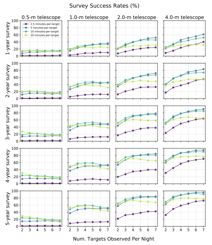
Figure 2: Survey success rates of different survey strategies. Telescope size increases to the right and survey duration from top to bottom. Each plot shows the percentage of surveys which were successful in detecting at least one planet for varying number of targets observed per night with different colours showing different observing times before slewing. Figure 6 from today’s paper.
The result is the optimal strategy is a 2m telescope, a survey duration of 3-4 years (assuming 120 nights per year with 30% time lost due to poor weather), 5-7 targets per night and slewing between targets every 5-10 minutes. This gave a 73-85% chance of detecting at least one 7.1 σ planet.
Practical limitations
There are some practical limitations not considered in the simulated survey but which could affect the results. Additional variability in the lightcurves can occur because large fractions of LTs are variable (0.2-0.4% over a few hours), and when dithering: if targets are not observed on the same part of the chip, the planet signal will be swamped. Another consideration is whether the period can be estimated from a single transit when you don’t have the full transit. While false positive signals, such as grazing eclipsing binaries, could be ruled out by mass estimation from spectra, LTs are unfortunately too faint to measure planet masses, meaning any planets can only be considered validated rather than confirmed.
Overall, the simulated survey found their optimal strategy had a good chance of detecting at least one planet and perhaps two in a four year survey. While these targets are of great interest, it is a large time investment for likely not many detections. However, this paper assumes planet occurrence rates the same as M dwarfs, which the authors postulate could be an underestimation, as planet occurrence rates increase from early to later M dwarfs. And as the ultracool dwarf TRAPPIST-1 has shown, one planetary system can make a big impact.
Author