Authors: Marc Hon, Daniel Huber, James S. Kuszlewicz, Dennis Stello, Sanjib Sharma, Jamie Tayar, Joel C. Zinn, Mathieu Vrard, and Marc H. Pinsonneault
First Author’s Institution: Institute for Astronomy, University of Hawai’i, Honolulu, Hawai’i, USA
Status: Published in the Astrophysical Journal [open access] (arXiv)
It’s no secret that machine learning has been incredibly useful in astronomy given the influx of large data sets. NASA’s Transiting Exoplanet Survey Satellite (TESS) has produced over 24 million light curves which correspond to over 14 million unique stars! Not only has TESS proved powerful in discovering exoplanets, it has also enabled great progress in stellar astrophysics. Asteroseismology – the study of stellar oscillations – has revolutionized stellar physics, and proved indispensable in measuring fundamental stellar properties. The more we learn about stars – for example, their composition, age, and other properties – the better we understand the Milky Way galaxy, and its formation and evolution. Therefore, authors of today’s paper leverage the power of machine learning to sift through millions of light curves and identify stars (specifically bright red giants) with solar-like oscillations.
Asteroseismology 101
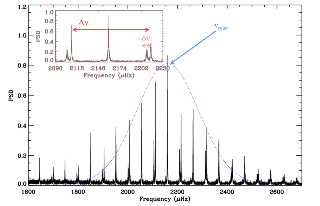
Asteroseismologists study sound waves bouncing within stars – driven by pressure and buoyancy – to study stellar interiors and composition. These oscillations can be seen in time-series photometry (changes in brightness over time). By converting the time-series data into the frequency domain, we can pick out frequencies at which a star is oscillating; these frequencies are referred to as oscillation modes. There are two main global frequencies used to derive fundamental stellar parameters that measure surface gravity and stellar density: frequency of maximum oscillation (\(\nu_{\textrm{max}}\)) and the large frequency spacing (\(\Delta \nu\)), respectively. In Figure 1, we see the power spectrum (density of power per frequency as a function of frequency) for 16 Cyg A, with \(\nu_{\textrm{max}}\) and \(\Delta \nu\) labelled. For more details about asteroseismology, see this post for more significant background, and these posts (E. Newton, E. Avallone, M. Sayeed) for additional descriptions.
The \(\Delta \nu\) quantity is difficult to measure for data with low-frequency resolution. Therefore, this paper only measured \(\nu_{\textrm{max}}\), and combined it with radius and temperature (measured independently) to calculate stellar mass.
Intro to Neural Networks
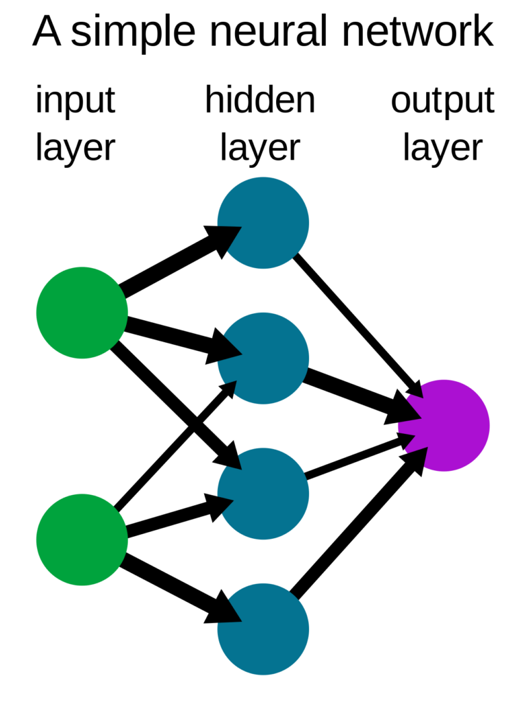
Machine learning can be classified into two major categories: supervised and unsupervised. In supervised learning, such as neural networks, a model is trained using a labelled data set, and is then refined to predict the output for a new data set. Briefly, a neural network (NN) utilises neurons to recognize patterns in a given data set, and mimics the way our brain uses billions of perceptrons with trillions of connections, to operate. Each neuron receives information in quantitative format, and its task is to perform a mathematical function on input data. In the instance of a 2D image in grayscale, the input data would be the brightness of a pixel represented by a number between 0 to 1 that is fed into a neuron, which takes the number and operates on it. For a 2D image, each neuron is responsible for finding and/or interpreting different aspects of the image. These are called ‘features’.
In addition, a neural network has at least three layers: input layer (which takes in the data), output layer and a hidden layer, and each of them can have more than one neuron. A neuron in a hidden layer takes the information from the input layer, operates on it, and passes information on to the next layer, which could be another hidden layer. For a more general overview, refer to this video on Neural Networks, and these bites (R. Golant, K. Gozman) for additional summaries.
Training the Model
In this paper, the authors implement two neural networks with two different goals: classification and regression. The first network takes a 2D image of the power spectrum and outputs a detection probability between 0 and 1 which represents the probability of detecting oscillations in a given spectrum. The second network (independent from the first) is a regression network that measures the frequency of maximum oscillation power (\(\nu_{\textrm{max}}\)). Given their implementation of supervised learning, they employed Kepler data for training, validation and testing, since \(\nu_{\textrm{max}}\) values are available for most red giants. To create a high-performance model, they trained their data on 196,581 Kepler light curves for their first neural network, and 16,194 red giants for their second neural network. The first NN included both oscillating and non-oscillating stars, while the second NN only included oscillating red giants. However, given their use of Kepler data for training, they also simulated noisier data to account for noise differences between Kepler and TESS data.
Map of the Sky

By training on stars which are known to be oscillating and have a measured \(\nu_{\textrm{max}}\), authors of this paper were able to derive \(\nu_{\textrm{max}}\) (and therefore surface gravity) for 158,505 red giants. When combined with radii estimated from Gaia, this has allowed them to estimate stellar masses and create the first near all-sky seismic mass map. Figure 3 shows the masses for nearly 140,000 stars across the sky. They find that higher mass stars are distributed in the Galactic disk, while lower mass stars occupy regions above and below the plane. This is consistent with our knowledge of Galaxy evolution; stars with higher masses are younger, and would be found in the galaxy’s thin disk.
This is the first time an all-sky map of seismic stellar masses has been created. The video below shows the locations of these stars across the sky as observed by TESS.
The authors of today’s paper have provided a preview of what astronomers can accomplish given the power of machine learning and large data sets. As more data are collected and more machine learning techniques are developed, the future of stellar astronomy looks extremely bright.
Edited by: Sahil Hegde
Featured image credit: NASA/MIT/TESS and Ethan Kruse (USRA)
Disclaimer: the writer’s previous advisor and group members are authors on this paper, but the writer was not involved in the work.